I have spent a few days hand-rolling neural networks such as CNN and RNN. This post shows my notes of neural network backpropagation derivation. The derivation of Backpropagation is one of the most complicated algorithms in machine learning. There are many resources for understanding how to compute gradients using backpropagation. But in my opinion, most of them lack a simple example to demonstrate the problem and walk through the algorithm.
1. A Simple Neural Network
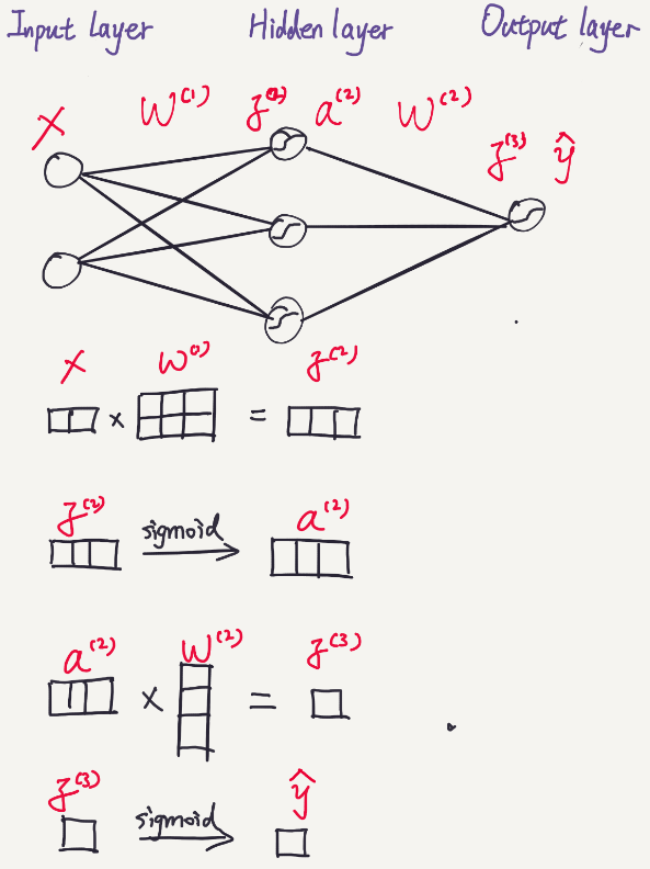
The following diagram shows the structure of a simple neural network used in this post. The input dimension (feature dimension) is 2, hidden layer size is 3, and the output dimension is 1. It is pretty intuitive to calculate the prediction by feeding forward the network. In the following diagram, instead of using real numbers, I use boxes to illustrate the dimension transformation through the layers.
2. Cost Function
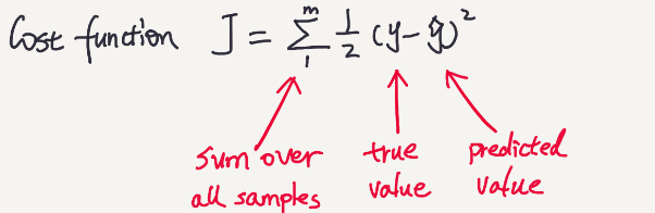
A cost function reflects the distance between the ground truth and the predicted values.A simple cost function is sum squared error function:
The cost J is a function of W. So the goal is to find the best W which yields the lowest cost J. The cost function is often defined in a way which is mathematically convenient. Apparently, there could be multiple ways to evaluate the distance between the truth and the predicted values. Each cost function has its own applicable cases. You may check out this post to see some other cost functions.
In a simplified two dimensional space, the relation between the cost J and W may look like:
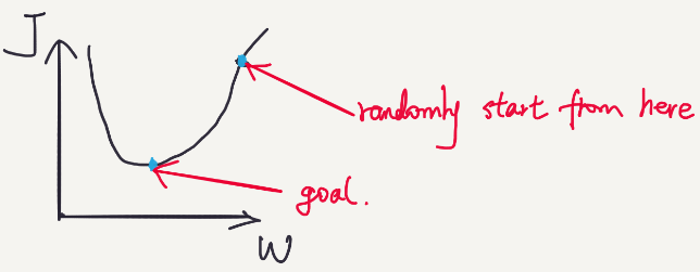
We keep updating W, so that the cost moves to the lowest point. The algorithm is called gradient descent. By calculating the partial derivatives of W, we can keep updating W and make the cost go lower and lower until reaching the lowest.
In a real scenario, it would be a multi-dimensional space (hard to visualize here). Each move will lead to a direction in a multi-dimensional space.
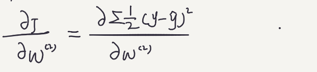
3. Partial Derivative Calculation
Let’s first calculate the partial derivatives of the second layer W.
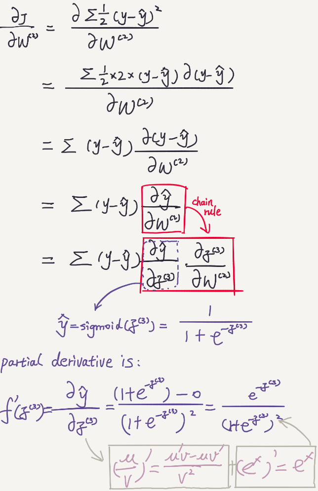
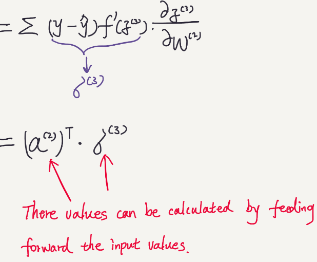
We can see that those values are only affected by the input data that is feed into the network. (Note that f'(z) can be further simplified.)
Similarly, we can calculate the partial derivatives of W for the first layer.
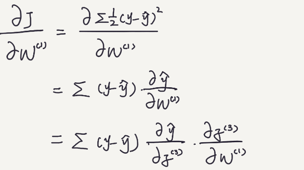
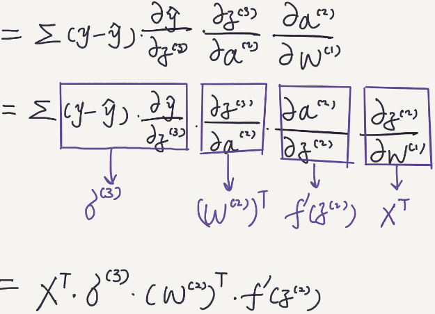
Those values are also can be calculated based on the input data that is feed into the network.
Once we know how to update W, we use the new W and do gradient descent over and over again, until reaching the optimal point.
4. Visualization of the Calculation
Let’s take the weights of the second layer for example.
We can see first how each sample contributes to the gradient, and then see how all 5 training samples contribute to the gradient.
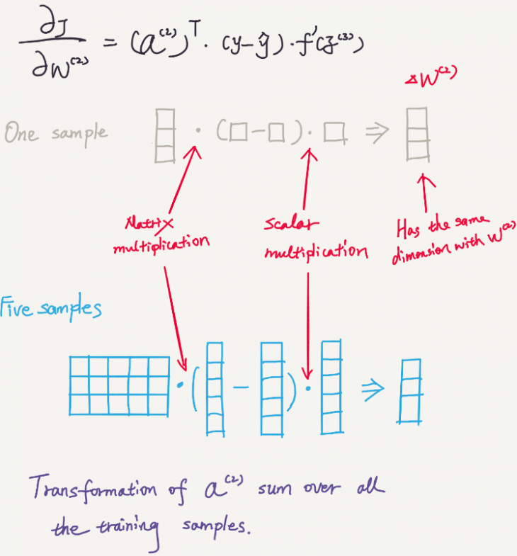
The dimension of the result is 3 by 1 which is the same of W2.
Thanks for explanation!