 |
 |
 |
 |
 |
 |
 |
 |
 |


![]()

![]()
![]()


Swarm Intelligence in Python
(Genetic Algorithm, Particle Swarm Optimization, Simulated Annealing, Ant Colony Algorithm, Immune Algorithm,Artificial Fish Swarm Algorithm in Python)
pip install scikit-optFor the current developer version:
git clone git@github.com:guofei9987/scikit-opt.git
cd scikit-opt
pip install .UDF (user defined function) is available now!
For example, you just worked out a new type of selection function.
Now, your selection function is like this:
-> Demo code: examples/demo_ga_udf.py#s1
# step1: define your own operator:
def selection_tournament(algorithm, tourn_size):
    FitV = algorithm.FitV
    sel_index = []
    for i in range(algorithm.size_pop):
        aspirants_index = np.random.choice(range(algorithm.size_pop), size=tourn_size)
        sel_index.append(max(aspirants_index, key=lambda i: FitV[i]))
    algorithm.Chrom = algorithm.Chrom[sel_index, :]  # next generation
    return algorithm.Chrom
Import and build ga
-> Demo code: examples/demo_ga_udf.py#s2
import numpy as np
from sko.GA import GA, GA_TSP

demo_func = lambda x: x[0] ** 2 + (x[1] - 0.05) ** 2 + (x[2] - 0.5) ** 2
ga = GA(func=demo_func, n_dim=3, size_pop=100, max_iter=500, lb=[-1, -10, -5], ub=[2, 10, 2],
        precision=[1e-7, 1e-7, 1])
Regist your udf to GA
-> Demo code: examples/demo_ga_udf.py#s3
ga.register(operator_name='selection', operator=selection_tournament, tourn_size=3)scikit-opt also provide some operators
-> Demo code: examples/demo_ga_udf.py#s4
from sko.operators import ranking, selection, crossover, mutation

ga.register(operator_name='ranking', operator=ranking.ranking). \
    register(operator_name='crossover', operator=crossover.crossover_2point). \
    register(operator_name='mutation', operator=mutation.mutation)
Now do GA as usual
-> Demo code: examples/demo_ga_udf.py#s5
best_x, best_y = ga.run()
print('best_x:', best_x, '\n', 'best_y:', best_y)
Until Now, the udf surport
crossover,mutation,selection,rankingof GA scikit-opt provide a dozen of operators, see here
For advanced users:
-> Demo code: examples/demo_ga_udf.py#s6
class MyGA(GA):
    def selection(self, tourn_size=3):
        FitV = self.FitV
        sel_index = []
        for i in range(self.size_pop):
            aspirants_index = np.random.choice(range(self.size_pop), size=tourn_size)
            sel_index.append(max(aspirants_index, key=lambda i: FitV[i]))
        self.Chrom = self.Chrom[sel_index, :]  # next generation
        return self.Chrom

    ranking = ranking.ranking

demo_func = lambda x: x[0] ** 2 + (x[1] - 0.05) ** 2 + (x[2] - 0.5) ** 2
my_ga = MyGA(func=demo_func, n_dim=3, size_pop=100, max_iter=500, lb=[-1, -10, -5], ub=[2, 10, 2],
        precision=[1e-7, 1e-7, 1])
best_x, best_y = my_ga.run()
print('best_x:', best_x, '\n', 'best_y:', best_y)We are developing GPU computation, which will be stable on version 1.0.0
An example is already available: https://github.com/guofei9987/scikit-opt/blob/master/examples/demo_ga_gpu.py
(New in version 0.3.6)
Run an algorithm for 10 iterations, and then run another 20 iterations base on the 10 iterations before:
from sko.GA import GA

func = lambda x: x[0] ** 2
ga = GA(func=func, n_dim=1)
ga.run(10)
ga.run(20)Step1:define your problem
-> Demo code: examples/demo_de.py#s1
'''
min f(x1, x2, x3) = x1^2 + x2^2 + x3^2
s.t.
    x1*x2 >= 1
    x1*x2 <= 5
    x2 + x3 = 1
    0 <= x1, x2, x3 <= 5
'''

def obj_func(p):
    x1, x2, x3 = p
    return x1 ** 2 + x2 ** 2 + x3 ** 2

constraint_eq = [
    lambda x: 1 - x[1] - x[2]
]

constraint_ueq = [
    lambda x: 1 - x[0] * x[1],
    lambda x: x[0] * x[1] - 5
]
Step2: do Differential Evolution
-> Demo code: examples/demo_de.py#s2
from sko.DE import DE

de = DE(func=obj_func, n_dim=3, size_pop=50, max_iter=800, lb=[0, 0, 0], ub=[5, 5, 5],
        constraint_eq=constraint_eq, constraint_ueq=constraint_ueq)

best_x, best_y = de.run()
print('best_x:', best_x, '\n', 'best_y:', best_y)
Step1:define your problem
-> Demo code: examples/demo_ga.py#s1
import numpy as np
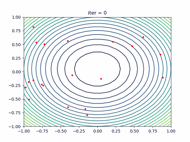
def schaffer(p):
'''
This function has plenty of local minimum, with strong shocks
global minimum at (0,0) with value 0
'''
x1, x2 = p
x = np.square(x1) + np.square(x2)
return 0.5 + (np.sin(x) - 0.5) / np.square(1 + 0.001 * x)
Step2: do Genetic Algorithm
-> Demo code: examples/demo_ga.py#s2
from sko.GA import GA

ga = GA(func=schaffer, n_dim=2, size_pop=50, max_iter=800, lb=[-1, -1], ub=[1, 1], precision=1e-7)
best_x, best_y = ga.run()
print('best_x:', best_x, '\n', 'best_y:', best_y)
Step3: plot the result
-> Demo code: examples/demo_ga.py#s3
import pandas as pd
import matplotlib.pyplot as plt

Y_history = pd.DataFrame(ga.all_history_Y)
fig, ax = plt.subplots(2, 1)
ax[0].plot(Y_history.index, Y_history.values, '.', color='red')
Y_history.min(axis=1).cummin().plot(kind='line')
plt.show()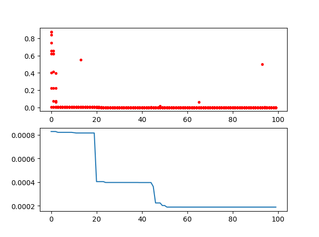
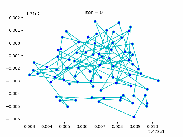
Just import the GA_TSP, it overloads the crossover, mutation to solve the TSP
Step1: define your problem. Prepare your points coordinate and the distance matrix.
Here I generate the data randomly as a demo:
-> Demo code: examples/demo_ga_tsp.py#s1
import numpy as np
from scipy import spatial
import matplotlib.pyplot as plt

num_points = 50

points_coordinate = np.random.rand(num_points, 2)  # generate coordinate of points
distance_matrix = spatial.distance.cdist(points_coordinate, points_coordinate, metric='euclidean')

def cal_total_distance(routine):
    '''The objective function. input routine, return total distance.
    cal_total_distance(np.arange(num_points))
    '''
    num_points, = routine.shape
    return sum([distance_matrix[routine[i % num_points], routine[(i + 1) % num_points]] for i in range(num_points)])
Step2: do GA
-> Demo code: examples/demo_ga_tsp.py#s2
from sko.GA import GA_TSP

ga_tsp = GA_TSP(func=cal_total_distance, n_dim=num_points, size_pop=50, max_iter=500, prob_mut=1)
best_points, best_distance = ga_tsp.run()
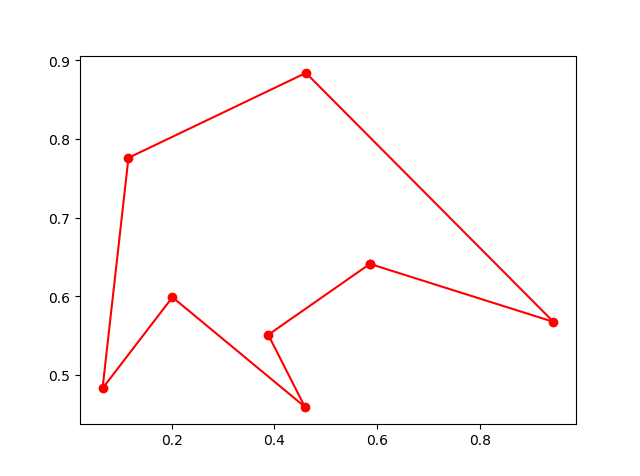
Step3: Plot the result:
-> Demo code: examples/demo_ga_tsp.py#s3
fig, ax = plt.subplots(1, 2)
best_points_ = np.concatenate([best_points, [best_points[0]]])
best_points_coordinate = points_coordinate[best_points_, :]
ax[0].plot(best_points_coordinate[:, 0], best_points_coordinate[:, 1], 'o-r')
ax[1].plot(ga_tsp.generation_best_Y)
plt.show()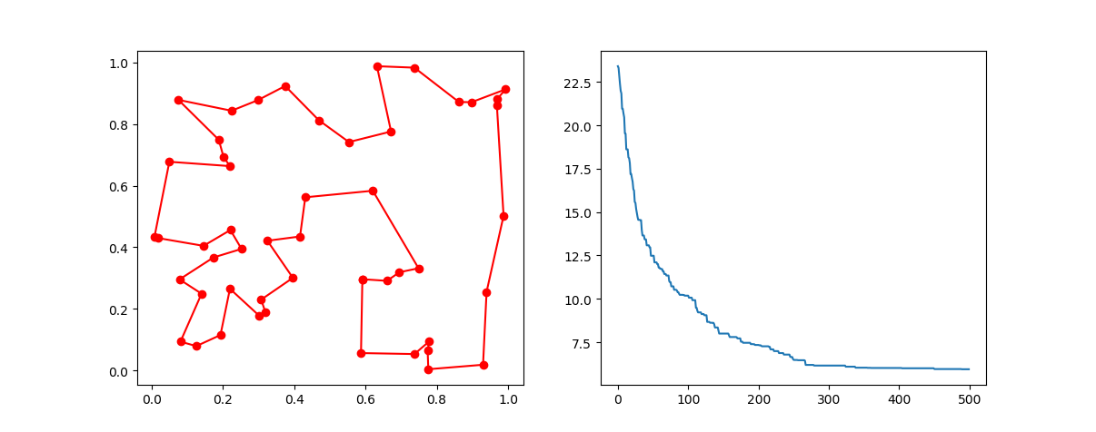
Step1: define your problem:
-> Demo code: examples/demo_pso.py#s1
def demo_func(x):
    x1, x2, x3 = x
    return x1 ** 2 + (x2 - 0.05) ** 2 + x3 ** 2
Step2: do PSO
-> Demo code: examples/demo_pso.py#s2
from sko.PSO import PSO

pso = PSO(func=demo_func, dim=3, pop=40, max_iter=150, lb=[0, -1, 0.5], ub=[1, 1, 1], w=0.8, c1=0.5, c2=0.5)
pso.run()
print('best_x is ', pso.gbest_x, 'best_y is', pso.gbest_y)
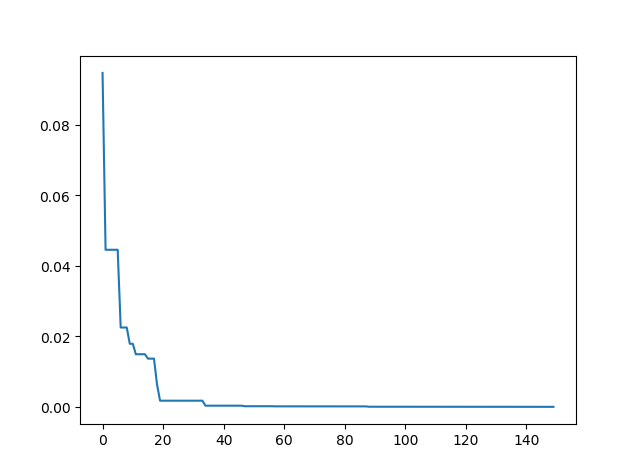
Step3: Plot the result
-> Demo code: examples/demo_pso.py#s3
import matplotlib.pyplot as plt

plt.plot(pso.gbest_y_hist)
plt.show()
-> Demo code: examples/demo_pso.py#s4
pso = PSO(func=demo_func, dim=3)
fitness = pso.run()
print('best_x is ', pso.gbest_x, 'best_y is', pso.gbest_y)Step1: define your problem
-> Demo code: examples/demo_sa.py#s1
demo_func = lambda x: x[0] ** 2 + (x[1] - 0.05) ** 2 + x[2] ** 2
Step2: do SA
-> Demo code: examples/demo_sa.py#s2
from sko.SA import SA

sa = SA(func=demo_func, x0=[1, 1, 1], T_max=1, T_min=1e-9, L=300, max_stay_counter=150)
best_x, best_y = sa.run()
print('best_x:', best_x, 'best_y', best_y)
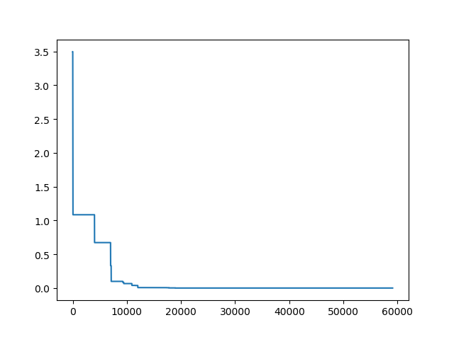
Step3: Plot the result
-> Demo code: examples/demo_sa.py#s3
import matplotlib.pyplot as plt
import pandas as pd

plt.plot(pd.DataFrame(sa.best_y_history).cummin(axis=0))
plt.show()
Moreover, scikit-opt provide 3 types of Simulated Annealing: Fast, Boltzmann, Cauchy. See more sa
Step1: oh, yes, define your problems. To boring to copy this step.
Step2: DO SA for TSP
-> Demo code: examples/demo_sa_tsp.py#s2
from sko.SA import SA_TSP

sa_tsp = SA_TSP(func=cal_total_distance, x0=range(num_points), T_max=100, T_min=1, L=10 * num_points)

best_points, best_distance = sa_tsp.run()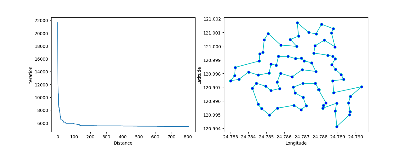
print(best_points, best_distance, cal_total_distance(best_points))Step3: plot the result
-> Demo code: examples/demo_sa_tsp.py#s3
from matplotlib.ticker import FormatStrFormatter
fig, ax = plt.subplots(1, 2)
best_points_ = np.concatenate([best_points, [best_points[0]]])
best_points_coordinate = points_coordinate[best_points_, :]
ax[0].plot(sa_tsp.best_y_history)
ax[0].set_xlabel("Iteration")
ax[0].set_ylabel("Distance")
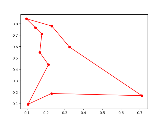
ax[1].plot(best_points_coordinate[:, 0], best_points_coordinate[:, 1],
marker='o', markerfacecolor='b', color='c', linestyle='-')
ax[1].xaxis.set_major_formatter(FormatStrFormatter('%.3f'))
ax[1].yaxis.set_major_formatter(FormatStrFormatter('%.3f'))
ax[1].set_xlabel("Longitude")
ax[1].set_ylabel("Latitude")
plt.show()
More: Plot the animation:
-> Demo code: examples/demo_aca_tsp.py#s2
from sko.ACA import ACA_TSP

aca = ACA_TSP(func=cal_total_distance, n_dim=num_points,
              size_pop=50, max_iter=200,
              distance_matrix=distance_matrix)

best_x, best_y = aca.run()
-> Demo code: examples/demo_ia.py#s2
from sko.IA import IA_TSP

ia_tsp = IA_TSP(func=cal_total_distance, n_dim=num_points, size_pop=500, max_iter=800, prob_mut=0.2,
                T=0.7, alpha=0.95)
best_points, best_distance = ia_tsp.run()
print('best routine:', best_points, 'best_distance:', best_distance)
-> Demo code: examples/demo_afsa.py#s1
def func(x):
    x1, x2 = x
    return 1 / x1 ** 2 + x1 ** 2 + 1 / x2 ** 2 + x2 ** 2

from sko.AFSA import AFSA

afsa = AFSA(func, n_dim=2, size_pop=50, max_iter=300,
            max_try_num=100, step=0.5, visual=0.3,
            q=0.98, delta=0.5)
best_x, best_y = afsa.run()
print(best_x, best_y)