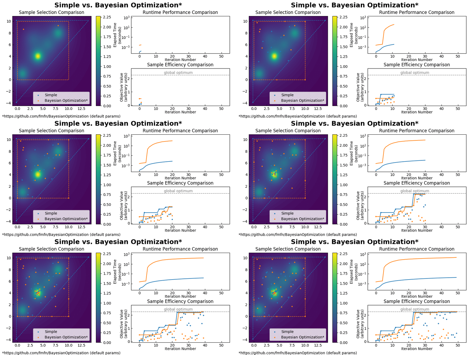
Simple is a radically more scalable alternative to Bayesian Optimization. Like Bayesian Optimization, it is highly sample-efficient, converging to the global optimum in as few samples as possible. Unlike Bayesian Optimization, it has a runtime performance of O(log(n)) instead of O(n^3) (or O(n^2) with approximations), as well as a constant factor that is roughly three orders of magnitude smaller. Simple's runtime performance, combined with its superior sample efficiency in high dimensions, allows the algorithm to easily scale to problems featuring large numbers of design variables.
For typical optimization workloads, the CPU time consumed by Bayesian Optimization is measured in minutes, while the CPU time used by Simple is measured in milliseconds. See for yourself:
 (Also you can find a comparison with CMA-ES here.)
Like Bayesian Optimization, Simple operates by constructing an internal surrogate model of the objective function's behavior. Both algorithms sample from points that their surrogate models predict to have a high objective value, as well as a large amount of information gain in order to make more accurate predictions in future iterations. Bayesian Optimization uses Gaussian processes to model the objective function, which, while they are very statistically rigorous, are also very computationally expensive.
Simple constructs its surrogate model by breaking up the optimization domain into a set of discrete, local interpolations that are independent from one another. Each of these local interpolations takes the form of a simplex, which is the mathematical term for the geometric concept of a triangle, but extended to higher dimensions. By testing a single point inside each simplex, the algorithm can split the parent interpolation into dim+1 smaller, more accurate child interpolations. A somewhat similar method for optimization using local simplicial interpolations and barycentric subdivision was first proposed by Wu, Ozdamar, and Kumar in 2005. Simple belongs to this same class of "space partitioning algorithms."
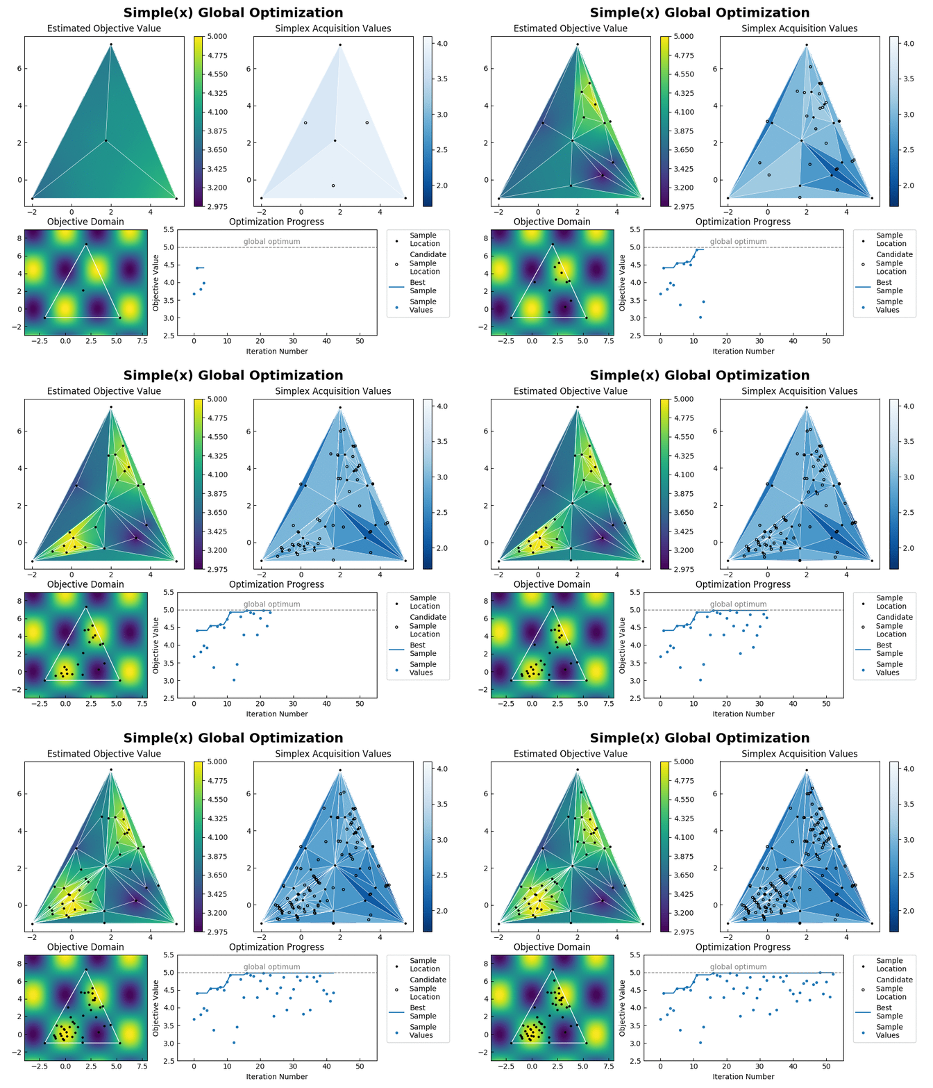
Simple achieves such an enormous speedup over Bayesian Optimization by transforming the global optimization problem into a dynamic programming problem. Since each interpolation is based on purely local information, individual samples can be taken without the need to recompute the updated surrogate model for the entire search space. At each step, Simple takes the local interpolation with the highest acquisition function value (the highest combined interpolated value and information gain) from its priority queue and evaluates the objective function at this interpolation's test point. The algorithm then uses the new sample information to subdivide the parent interpolation into smaller child interpolations, which it proceeds to add back to the priority queue. Here is a view of the algorithm in action:

Each simplex has a candidate test location that is determined geometrically to help guarantee convergence and inhibit the creation of less accurate high aspect ratio interpolations. In more detail, the acquisition function is given by acquisition = interpolated_value + exploration_preference * opportunity_cost. The exploration preference is an adjustable hyperparameter that is used to inform the algorithm how much importance it should give to exploring the optimization domain, as opposed to pursuing the first local optimum that it finds.
Inverse distance weighting is used to interpolate the objective value across each simplex from its vertices. The opportunity cost is a relative measure of how much each region of space containing a candidate test point has already been explored. This is determined by opportunity_cost = (best_sample - worst_sample) * log(parent_area_fraction * child_area_coordinate) where log is the dim+1 base logarithm. When subdividing a regular simplex of dimensiion dim, it will be split into dim+1 simplexes each with content that is 1/(dim+1) of the parent simplex. Thus the opportunity cost calculation is represetative of how many times a regularly shaped simplex of equivalent content would have already been sampled.
First, pip install numpy matplotlib, then place Simple.py in the same working directory as your code. Once that is done you can try the following:
from Simple import SimpleTuner

objective_function = lambda vector: -((vector[0] - 0.2) ** 2.0 + (vector[1] - 0.3) ** 2.0) ** 0.5
optimization_domain_vertices = [[0.0, 0.0], [0, 1.0], [1.0, 0.0]]
number_of_iterations = 30
exploration = 0.05 # optional, default 0.15

tuner = SimpleTuner(optimization_domain_vertices, objective_function, exploration_preference=exploration)
tuner.optimize(number_of_iterations)
best_objective_value, best_coords = tuner.get_best()

print('Best objective value ', best_objective_value)
print('Found at sample coords ', best_coords)
tuner.plot() # only works in 2D
The resulting output is then:
Best objective value  -0.00823447695587
Found at sample coords [ 0.19285289 0.29591033]There are three minor caveats to this algorithm:
Simple works by constructing local interpolations between sets of sample points, which implies that there must be a sample taken at every corner point of the optimization domain. A prism-shaped optimization domain has 2^dim corner points, while a simplex-shaped domain possesses only dim+1 corner points. Therefore, a simplex-shaped optimization domain is the most sample-efficient choice for this algorithm, and allows it to efficiently optimize highly dimensional objective functions.
So while Simple does possess a hard requirement of needing to sample dim+1 corner points before optimization can proceed, this is actually an improvement when compared to the typical behavior of Bayesian Optimization. Bayesian Optimization usually operates on prism-shaped domains, and in practice has an overwhelming preference to sample the 2^dim corner points of its optimization domain since these tend to represent the most unexplored regions of the search space. In 10D, Simple only needs to test 11 corner points while Bayesian Optimization needs to sample 1024.
A few features got left out of this proof of concept release, mostly concerning guarantees for convergence with objective functions that plateau near their global optimum. These include enforcing a peak opportunity cost penalty, as well as transforming the values recieved from the objective function. Simple can also be extended to solve MINLP problems.
If there is enough interest, I plan to do a proper rewrite in C with strong support for parallel objective function evaluations, suitable for large-scale optimization in HPC applications.
If you like this work, I am seeking employment.