This repository provides the framework for the training, testing, analysis, and comparison of uncertainty quantification in 3D segmentations via Monte Carlo dropout networks and novel Bayesian convolutional neural networks (BCNNs). BCNNs leverage the TensorFlow Probability library to learn distributions over the weights, thus performing actual Bayesian inference by learning a posterior distribution rather than approximating one like Monte Carlo dropout. Our BCNN is the first-ever Bayesian CNN with variational inference in 3D. Paper here.
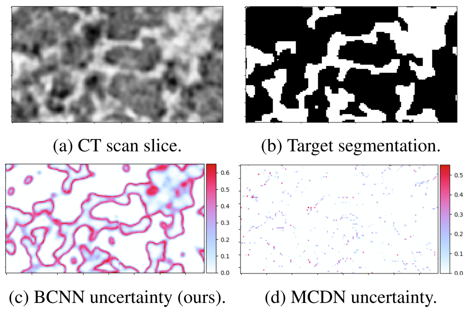
conda environment with conda create -n bcnn python==3.6.7pip install -r requirements.txtpython generate_toy_data.py"num_gpus"=1 and batch_size=2 in configs/toy_config.json (it's at the bottom)./toy_train_test.sh. This shell file "chunks" the large volumes and trains both a Bayesian and Monte Carlo dropout network, then compares the two on the test set. It saves model weights, prediction arrays, and sample images. In particular, check out the toy_images/*/*_unc.png images to see the differences in the uncertainty quantification output from both models. The BCNN and MCDN give approximately equivalent UQ in the toy example, but as the domains become more difficult, the BCNN achieves a clearly superior UQ performance. If you get an out-of-memory error, reduce the "batch_size" in configs/toy_config.json, delete toy_data, and start from Step 4.3D data is a bit hard to work with, but this repo streamlines the process. We "chunk" large volumes into a manageable size by scanning them with a rectangular prism window, then reconstructing the original volume during inference time.
config.json expects data directories to be specified in the orig* variables. This is where the original large volumes are contained. The user provides whether they want to standardize the data (norm), how much overlap they want (step), and how big the window should be (window).
Data will be automatically extracted and chunked according to these config values when train.py is called.
This repo provides 4 choices of models for experimentation. There is a 2D and 3D version of both the Monte Carlo dropout network and the BCNN. Specify which model you would like to use by setting the vnet and bayesian variables in config.json. It defaults to the 3D BCNN.
One can also set model hyperparameters, including prior_std, kernel_size, activation, etc. in config.json.
To train a model, first ensure that you have the correct data_dir and weights_dir variables set in config.json. If there is a saved model in weights_dir, it will resume with the most recently edited weights file by default. If you want to disable resuming, set resume to False; if you want to resume from a specific weights file, set weights_path. By default, tf.keras does not save the epoch with the weights, so set initial_epoch if you want to resume from a specific epoch (useful because learning rate is determined by epoch). Finally, one can also set training hyperparameters such as batch_size and num_gpus. As an example,
python train.py with configs/toy_config.json "data_dir"="mydata" "num_gpus"=2 "batch_size"=32 "prior_std"=1.5
Testing a model works much the same as training, with the additional impact of Monte Carlo samples. Depending on the variance of your model, you may need different amounts of samples. I found 5-10 to work for dropout models and ~30 to work for BCNNs. test.py will save the predictions and a few image slices automatically, so ensure to specify predict_dir and images_dir. As an example,
python test.py with configs/toy_config.json "bayesian"=False "mc_samples"=12 "weights_path"="model.h5"