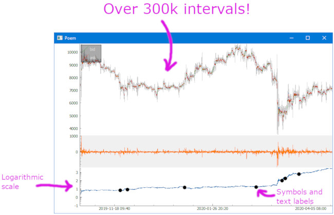
Finance Plot

Finance Plotter, or finplot, is a performant library with a clean api to help you with your backtesting. It's optionated with good defaults, so you can start doing your work without having to setup plots, colors, scales, autoscaling, keybindings, handle panning+vertical zooming (which all non-finance libraries have problems with). And best of all: it can show hundreds of thousands of datapoints without batting an eye.

Features

Great performance compared to mpl_finance, plotly and Bokeh
Clean api
Works with both stocks as well as cryptocurrencies on any time resolution
Show as many charts as you want on the same time axis, zoom on all of them at once
Auto-reload position where you were looking last run
Overlays, fill between, value bands, symbols, labels, legend, etc.
Can show real-time updates.

feature1 feature2 feature3

What it is not

finplot is not a web app. It does not help you create an homebrew exchange. It does not work with Jupyter Labs. It does not have a save screen shot function. It only shows time-based charts, i.e. no order depth, no trades, no tickers.

It is only intended for you to do backtesting in. That is not to say that you can't create these things yourself. The library is based on the eminent pyqtgraph, which is fast and flexible, so feel free to hack away if that's what you want.

Easy installation

$ pip install finplot

Example

It's straight-forward to start using. This shows every daily candle of Apple since the 80'ies:

import finplot as fplt
import yfinance

df = yfinance.download('AAPL')
fplt.candlestick_ochl(df[['Open', 'Close', 'High', 'Low']])
fplt.show()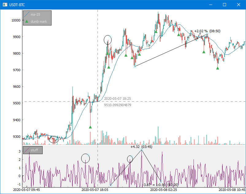

Example 2

sample

This 25-liner pulls some BitCoin data off of Bittrex and shows the above:

import finplot as fplt
import numpy as np
import pandas as pd
import requests

# pull some data
symbol = 'USDT-BTC'
url = 'https://bittrex.com/Api/v2.0/pub/market/GetTicks?marketName=%s&tickInterval=fiveMin' % symbol
data = requests.get(url).json()

# format it in pandas
df = pd.DataFrame(data['result'])
df = df.rename(columns={'T':'time', 'O':'open', 'C':'close', 'H':'high', 'L':'low', 'V':'volume'})
df = df.astype({'time':'datetime64[ns]'})

# create two plots
ax,ax2 = fplt.create_plot(symbol, rows=2)

# plot candle sticks
candles = df[['time','open','close','high','low']]
fplt.candlestick_ochl(candles, ax=ax)

# overlay volume on the top plot
volumes = df[['time','open','close','volume']]
fplt.volume_ocv(volumes, ax=ax.overlay())

# put an MA on the close price
fplt.plot(df['time'], df['close'].rolling(25).mean(), ax=ax, legend='ma-25')

# place some dumb markers on low wicks
lo_wicks = df[['open','close']].T.min() - df['low']
df.loc[(lo_wicks>lo_wicks.quantile(0.99)), 'marker'] = df['low']
fplt.plot(df['time'], df['marker'], ax=ax, color='#4a5', style='^', legend='dumb mark')

# draw some random crap on our second plot
fplt.plot(df['time'], np.random.normal(size=len(df)), ax=ax2, color='#927', legend='stuff')
fplt.set_y_range(-1.4, +3.7, ax=ax2) # hard-code y-axis range limitation

# restore view (X-position and zoom) if we ever run this example again
fplt.autoviewrestore()

# we're done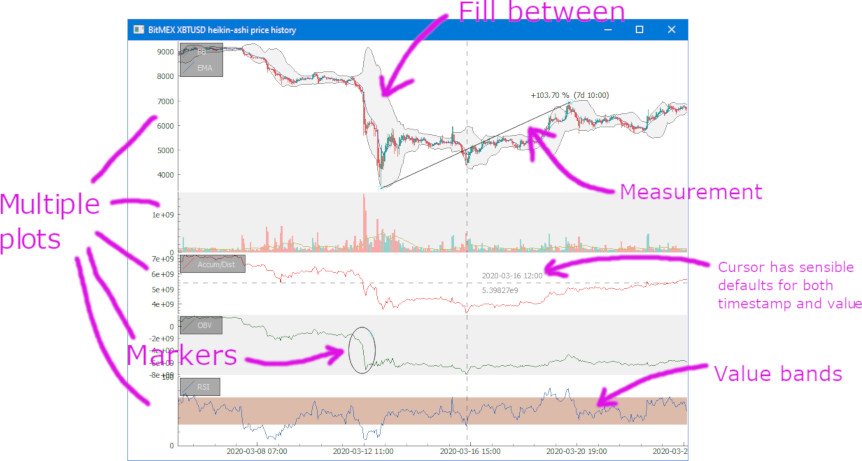
fplt.show()

Realtime updating with realistic indicator

Included in this repo are a 40-liner Bitfinex example and a slightly longer BitMEX websocket example, which both update in realtime with Bitcoin/Dollar pulled from the exchange. They also shows realistic and useful indicators (TD Sequential for BFX and Bollinger Bands for BitMEX). The S&P500 example shows you how to display MACD.

Enjoy!