What is Pytim | Examples | More info | How to Install | References


![]()

![]()
Disclaimer: Pytim is in beta-stage right now and while a systematic testing system has been set up, this has not yet total coverage. We will keep rolling out more examples and, still, some new features. If you try this software out and have some suggestions, remarks, or bugfixes, feel free to comment here on GitHub and/or make a pull request.
Jupyter Notebooks with more examples are available at Marcello-Sega/pytim-notebooks
The paper about pytim has been published on J. Comput. Chem. It is open access and you can download the pdf from Wiley  (see also the references)
Pytim is a cross-platform python implementation of several methods for the detection of fluid interfaces in molecular simulations. It is based on MDAnalysis, but it integrates also seamlessly with MDTraj, and can be even used for online analysis during an OpenMM simulation (see further down for examples with MDTraj and with OpenMM).
So far the following interface/phase identification methods have been implemented:

Pytim relies on the MDAnalysis package for reading/writing trajectories, and work therefore seamlessly for a number of popular trajectory formats, including:
as well as common structure file formats such as XYZ or PDB (have a look at the complete list)

PyPi: pip install --user --upgrade pytim
Anaconda: conda install -c conda-forge pytim
NOTE: on Mac OS you might want to use CFLAGS='-stdlib=libc++' pip install --user --upgrade pytim
Ok, ok ... have a look below: this example is about computing molecular layers of a flat interface:
import MDAnalysis as mda
import pytim
from pytim.datafiles import WATER_GRO

# load the configuration in MDAnalysis
u = mda.Universe(WATER_GRO)

# compute the interface using ITIM. Identify 4 layers.
inter = pytim.ITIM(u,max_layers=4)Now interfacial atoms are accessible in different ways, pick the one you like:
atoms group accessible asinter.atoms.positions # this is a numpy array holding the position of atoms in the layersarray([[ 22.10000038, 16.05999947, 94.19633484],
[ 22.43999863, 16.97999954, 93.96632385],
...,
[ 33.70999908, 49.02999878, 62.52632904],
[ 34.06999969, 48.18000031, 61.16632843]], dtype=float32)MDAnalysis universe now has, which specifies in which layer it is found: u.atoms.layers # -1 if not in any layer, 1 if in the first layer, ...inter.layers
array([[<AtomGroup with 780 atoms>, <AtomGroup with 690 atoms>,
<AtomGroup with 693 atoms>, <AtomGroup with 660 atoms>],
[<AtomGroup with 777 atoms>, <AtomGroup with 687 atoms>,
<AtomGroup with 663 atoms>, <AtomGroup with 654 atoms>]], dtype=object)Pytim can export in different file formats: the PDB format with the beta field used to tag the layers, VTK, cube for both continuous surfaces and particles, and, of course, all formats supported by MDAnalysis.
In VMD, for example, using beta == 1 allows you to select all atoms in the first interfacial layer. Just save your PDB file with layers information using
inter.writepdb('myfile.pdb')In a jupyter notebook, you can use nglview like this:
import nglview
v = nglview.show_mdanalysis(u)
v.camera='orthographic'
v.center()
system = v.component_0
colors = ['','red','orange','yellow','white']

for n in [1,2,3,4]:
    system.add_spacefill(selection = inter.atoms[inter.atoms.layers==n].indices, color=colors[n] )

system.add_spacefill(selection = (u.atoms - inter.atoms).indices, color='gray' )
# this must go in a separate cell
v.display()

MDAnalysis and mdtraj)Once one of the pytim classes (ITIM,GITIM,WillardChandler,...) has been initialised, whenever a new frame is loaded, the interfacial properties will be calculated automatically without need of doing anything else
import MDAnalysis as mda
import pytim
from pytim.datafiles import WATER_GRO, WATER_XTC

u = mda.Universe(WATER_GRO,WATER_XTC)
inter = pytim.ITIM(u)
for step in u.trajectory[:]:
print "surface atoms:", repr(inter.atoms)Under the hood, pytim uses MDAnalysis, but this is made (almost completely) transparent to the user, so that interoperability with other software is easy to implement. For example, to analyse a trajectory loaded with MDTraj, it is enough to do the following:
import mdtraj
import pytim
from pytim.datafiles import WATER_GRO, WATER_XTC

t = mdtraj.load_xtc(WATER_XTC,top=WATER_GRO)
inter = pytim.ITIM(t)
for step in t[:]:
print "surface atoms:" , repr(inter.atoms.indices)Another example is using pytim to perform online interfacial analysis during an OpenMM simulation:
# openmm imports
from simtk.openmm.app import *
from simtk.openmm import *
from simtk.unit import *
# pytim
import pytim
from pytim.datafiles import WATER_PDB

# usual openmm setup, we load one of pytim's example files
pdb = PDBFile(WATER_PDB)
forcefield = ForceField('amber99sb.xml', 'spce.xml')
system = forcefield.createSystem(pdb.topology, nonbondedMethod=PME,
        nonbondedCutoff=1*nanometer)
integrator = LangevinIntegrator(300*kelvin, 1/picosecond, 0.002*picoseconds)
simulation = Simulation(pdb.topology, system, integrator)
simulation.context.setPositions(pdb.positions)

# just pass the openmm Simulation object to pytim
inter = pytim.ITIM(simulation)
print repr(inter.atoms)

# the new interfacial atoms will be computed at the end
# of the integration cycle
simulation.step(10)
print repr(inter.atoms)
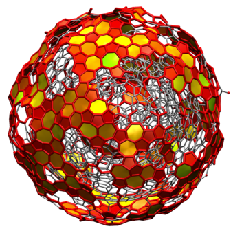
You could use GITIM, or the Willard-Chandler method. Let's have a look first at GITIM:
import MDAnalysis as mda
import pytim
from   pytim.datafiles import *

u       = mda.Universe(MICELLE_PDB)
g       = u.select_atoms('resname DPC')

interface = pytim.GITIM(u,group=g,molecular=False,
                        symmetry='spherical',alpha=2.5)
layer = interface.layers[0]
interface.writepdb('gitim.pdb',centered=False)
print repr(layer)
<AtomGroup with 872 atoms>
nglview can be used to show a section cut of the micelle in a jupyter notebook:
import nglview
import numpy as np

v = nglview.show_mdanalysis(u)
v.camera='orthographic'
v.center()
v.add_unitcell()
system = v.component_0
system.clear()

selection = g.atoms.positions[:,2]>30.
system.add_spacefill(selection =g.atoms.indices[selection])

selection = np.logical_and(inter.atoms.layers==1,inter.atoms.positions[:,2]>30.)
system.add_spacefill(selection =inter.atoms.indices[selection], color='yellow' )
v.display()

The Willard-Chandler method can be used, instead to find out isodensity surfaces:
import MDAnalysis as mda
import pytim
from pytim.datafiles import MICELLE_PDB
import nglview

u = mda.Universe(MICELLE_PDB)
g = u.select_atoms('resname DPC')
interface = pytim.WillardChandler(u, group=g, mesh=1.5, alpha=3.0)
interface.writecube('data.cube')Done, the density file is written in .cube format, we can now open it with
programs such as Paraview, or visualize it in a
jupyter notebook with nglview
view = nglview.show_mdanalysis(u.atoms) # the atoms, this will be component_0 in nglview
view.add_component('data.cube') # the density data, this will be component_1 in nglview

view.clear() # looks like this is needed in order for view._display_image() to work correctly
# let's center the view on our atoms, and draw them as spheres
view.component_0.center()
view.component_0.add_spacefill(selection='DPC')

# let's add a transparent, red representation for the isodensity surface at 50% density
view.component_1.add_surface(color='red',isolevelType="value",isolevel=0.5,opacity=0.6)

# add a nice simulation box
view.add_unitcell()
view.display()

import MDAnalysis as mda
import pytim
from   pytim.datafiles import GLUCOSE_PDB

u       = mda.Universe(GLUCOSE_PDB)
solvent = u.select_atoms('name OW')
glc     = u.atoms - solvent.residues.atoms

inter = pytim.GITIM(u, group=solvent, molecular=True,
                    max_layers=3, alpha=2)

for i in [0,1,2]:
    print "Layer "+str(i),repr(inter.layers[i])
Layer 0 <AtomGroup with 81 atoms>
Layer 1 <AtomGroup with 186 atoms>
Layer 2 <AtomGroup with 240 atoms>import nglview
import numpy as np
v = nglview.show_mdanalysis(u)
v.camera='orthographic'
v.center()
v.add_unitcell()
v.clear()
# glucose
v.add_licorice(selection =glc.atoms.indices,radius=.35)
colors = ['yellow','blue','purple']
# hydration layers
for layer in [0,1,2]:
selection = np.logical_and(inter.atoms.layers==layer+1 ,inter.atoms.positions[:,2]>9)
v.add_spacefill(selection =inter.atoms.indices[selection], color=colors[layer] )
v.display()

When calculating surfaces with GITIM, it can happen that several disconnected, closed surfaces are found in a simulation box. To restrict the analysis to the largest, clustered interfacial atoms (also when calculating multiple layers), one can pass the biggest_cluster_only option, as in:
inter = pytim.GITIM(u, group=solvent, molecular=True, max_layers=3, alpha=2,
                    biggest_cluster_only=True, cluster_cut = 3.5)
In order for this option to have any effect, a cluster_cut value should also be passed.
Have a look at the jupyter notebooks: https://github.com/Marcello-Sega/pytim-notebooks
Browse the examples in the Pytim Online Manual
Check out the Pytim Poster from the 10th Liquid Matter Conference Available on ResearchGate DOI:10.13140/RG.2.2.18613.17126
this will install the latest release present in the Python Package Index:
pip install --user --upgrade pytimpip install --user --upgrade cython numpy scipy MDAnalysisgit clone https://github.com/Marcello-Sega/pytim.git
cd pytim
python setup.py install --userPYTHONPATH variableIf you install with the option --user (which you have to do if you don't have administrator rights) you shouldn't forget to tell python where to look for the module by setting the PYTHONPATH environment variable.
Under Linux, you could do, for example:
export PYTHONPATH=$HOME/.local/lib/python2.7/site-packagesUnder OS-X, instead, use something like:
export PYTHONPATH=$HOME/Library/Python/2.7/lib/python/site-packagesYou can search for the exact path by issuing the following command:
python -c "import site; print(site.USER_SITE)"If this for some reason doesn't work, get some hint using:
find $HOME -name site-packagesSome of the most common issues are the following:
Problem: The system does not let me write (even using sudo) some files
Solution: You're most likely running under a recent version of OS-X. Always install packages as user (pip install <package> --user
Problem: cKDTree complains about the boxsize parameter
Solution: the version of scipy must be >= 0.18
Problem: Even though I've upgraded scipy, I keep getting problems about boxsize
Solution: You should tell python where to find packages by setting the variable $PYTHONPATH
Problem: some error message mentioning ... file was built for x86_64 which is not the architecture being linked (i386)
Solution: use export ARCHFLAGS='-arch x86_64' before installing
Problem: I'm getting an annoying message like "UserWarning: Module pytim_dbscan was already imported from [...]"
Solution: You've installed pytim, and are launching python within the pytim package directory. Move away from there :)
The pytim paper is avaliable (under the terms of the Creative Commons BY-NC 4.0 licence) from Wiley. Please cite it if you use pytim for your research:
M. Sega, S. G. Hantal, B. Fabian and P. Jedlovszky, J. Comp. Chem. 39, 2118-2125 (2018) Pytim: A python package for the interfacial analysis of molecular simulations
@article{sega2018pytim,
  title={Pytim: A python package for the interfacial analysis of molecular simulations},
  author={Sega, M. and Hantal, G. and F{\'a}bi{\'a}n, B. and Jedlovszky, P.},
  journal={J. Comput. Chem.},
  pages={2118--2125},
  volume={39},
  year={2018},
  publisher={Wiley Online Library}
}
Depending on which algorithm you are using, you might also want to cite the following:
M. Sega, S. S. Kantorovich, P. Jedlovszky and M. Jorge, J. Chem. Phys. 138, 044110 (2013) The generalized identification of truly interfacial molecules (ITIM) algorithm for nonplanar interfaces.
L. B. Pártay, G. Hantal, P. Jedlovszky, Á. Vincze and G. Horvai, J. Comp. Chem. 29, 945 (2008) A new method for determining the interfacial molecules and characterizing the surface roughness in computer simulations. Application to the liquid–vapor interface of water
M. Sega and G. Hantal.Phys. Chem. Chem. Phys. 29, 18968-18974 (2017) Phase and interface determination in computer simulations of liquid mixtures with high partial miscibility.
E. Chacón, P. Tarazona, Phys. Rev. Lett. 91, 166103 (2003) Intrinsic profiles beyond the capillary wave theory: A Monte Carlo study.
A. P. Willard, D. Chandler, J. Phys. Chem. B 114,1954 (2010) Instantaneous Liquid Interfaces