Senin, Pavel and Malinchik, Sergey, SAX-VSM: Interpretable Time Series ClassiCfication Using SAX and Vector Space Model, Data Mining (ICDM), 2013 IEEE 13th International Conference on, pp.1175,1180, 7-10 Dec. 2013.
[1] Lin, J., Keogh, E., Wei, L. and Lonardi, S., Experiencing SAX: a Novel Symbolic Representation of Time Series. DMKD Journal, 2007.
[2] Salton, G., Wong, A., Yang., C., A vector space model for automatic indexing. Commun. ACM 18, 11, 613–620, 1975.
[3] Jones, D. R. , Perttunen, C. D., and Stuckman, B. E., Lipschitzian optimization without the lipschitz constant, Journal of Optimization Theory and Applications, vol. 79, no. 1, pp. 157–181, 1993
[4] The DiRect implementation source code is partially based on JCOOL.
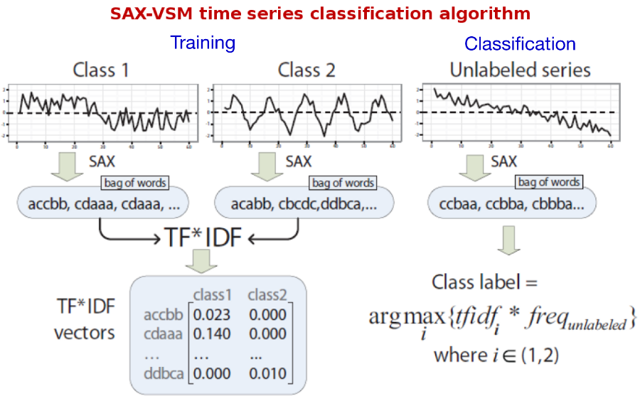
The proposed interpretable time series classification algorithm consists of two steps -- training and classification.
For training, labeled time series discretized with SAX via sliding window and "bag of words" constructed for each of the training classes (single bag per class). Processing bags with TFIDF yields a set of class-characteristic vectors -- one vector per class. Essentially, each element of that vector is a weighted discretized fragment of the input time series whose weight value reflects its "class-characteristic power" and the class specificity.
For classification, the unlabeled time series is discretized with sliding window-based SAX (exactly the same transform as for training) in order to transform it into a term frequency vector. Next, the cosine similarity computed between this vector and those constructed during training (i.e., vectors characterizing training classes). The unlabeled input time series assigned to a class with which the angle is smallest, i.e., the cosine value is largest. This is ltc.nnn schema in SMART notation.
Because it is easy to see which patterns contribute the most to the cosine similarity value, as well as to see which patterns have the highest weights after training, the algorithm naturally enables the interpretation of training and classification results.
The whole process is illustrated below:
The code is written in Java and I use maven to build it:
$ mvn package -P single
[INFO] Scanning for projects...
[INFO] ------------------------------------------------------------------------
[INFO] Building sax-vsm
[INFO]    task-segment: [package]
...
[INFO] Building jar: /media/Stock/git/sax-vsm_classic.git/target/sax-vsm-0.0.1-SNAPSHOT-jar-with-dependencies.jar
[INFO] ------------------------------------------------------------------------
[INFO] BUILD SUCCESSFULClass SAXVSMClassifier is runnable from command line; running it without parameters prints usage help. Here is a trace of running SAX-VSM with Gun/Point dataset:
$ java -cp "target/sax-vsm-0.0.1-SNAPSHOT-jar-with-dependencies.jar" net.seninp.jmotif.SAXVSMClassifier \
  -train src/resources/data/Gun_Point/Gun_Point_TRAIN -test src/resources/data/Gun_Point/Gun_Point_TEST \
  -w 33 -p 17 -a 15
trainData classes: 2, series length: 150
 training class: 2 series: 26
 training class: 1 series: 24
testData classes: 2, series length: 150
 test class: 2 series: 74
 test class: 1 series: 76
classification results: strategy EXACT, window 33, PAA 17, alphabet 15, accuracy 1.00, error 0.00Symbolic discretization with SAX -- the first step of our algorithm -- requires hyperparameters to be specified by the user. Unfortunately, their optimal selection is not trivial. We proposed to use Dividing Rectangles optimization scheme for accelerated selection of optimal parameter values.
The code implements the DiRect sampler which can be called from the command line. Below is the trace of running the sampler for Gun/Point dataset. The series in this dataset have length 150, so I define the sliding window range as [10-150], PAA size as [5-75], and the alphabet [2-18]:
$ java -jar target/sax-vsm-0.0.1-SNAPSHOT-jar-with-dependencies.jar \
-train src/resources/data/Gun_Point/Gun_Point_TRAIN -test src/resources/data/Gun_Point/Gun_Point_TEST \
-wmin 10 -wmax 150 -pmin 5 -pmax 75 -amin 2 -amax 18 --hold_out 1 -i 3
trainData classes: 2, series length: 150
training class: 2 series: 26
training class: 1 series: 24
testData classes: 2, series length: 150
test class: 2 series: 74
test class: 1 series: 76
running sampling for MINDIST strategy...
iteration: 0, minimal value 0.18 at 80, 40, 10
iteration: 1, minimal value 0.04 at 80, 17, 10
iteration: 2, minimal value 0.04 at 80, 17, 10
min CV error 0.04 reached at [80, 17, 10], will use Params [windowSize=80, paaSize=17, alphabetSize=10, nThreshold=0.01, nrStartegy=MINDIST]
running sampling for EXACT strategy...
iteration: 0, minimal value 0.0 at 80, 40, 10
iteration: 1, minimal value 0.0 at 80, 40, 10
iteration: 2, minimal value 0.0 at 80, 40, 10
min CV error 0.00 reached at [80, 40, 10], [33, 17, 15], will use Params [windowSize=33, paaSize=17, alphabetSize=15, nThreshold=0.01, nrStartegy=EXACT]
running sampling for NONE strategy...
iteration: 0, minimal value 0.0 at 80, 40, 10
iteration: 1, minimal value 0.0 at 80, 40, 10
iteration: 2, minimal value 0.0 at 80, 40, 10
min CV error 0.00 reached at [80, 40, 10], [64, 40, 10], [33, 17, 15], will use Params [windowSize=33, paaSize=17, alphabetSize=15, nThreshold=0.01, nrStartegy=NONE]
classification results: strategy MINDIST, window 80, PAA 17, alphabet 10, accuracy 0.92667, error 0.07333
classification results: strategy EXACT, window 33, PAA 17, alphabet 15, accuracy 1.00, error 0.00
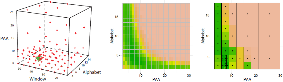
classification results: strategy NONE, window 33, PAA 17, alphabet 15, accuracy 0.97333, error 0.02667As shown in our work, DiRect provides a significant speed-up when compared with the grid search. Below is an illustration of DiRect-driven parameters optimization for SyntheticControl dataset. Left panel shows all points sampled by DiRect in the space PAA ∗ W ndow ∗ Alphabet: red points correspond to high error values while green points correspond to low error values in cross-validation experiments. Note the green points concentration at W=42 (where the optimal value is). Middle panel shows the classification error heat map obtained by a complete scan of all 432 points of the hypercube slice when W=42. Right panel shows the classification error heat map of the same slice when the parameters search optimized by DiRect, the optimal solution (P=8,A=4) was found by sampling of 43 points (i.e., 10X speed-up for the densily sampled slice).
The class named SAXVSMPatternExplorer prints the most significant class-characteristic patterns, their weights, and the time-series that contain those. The best_words_heat.R script allows to plot these. Here is an example for the Gun/Point data:
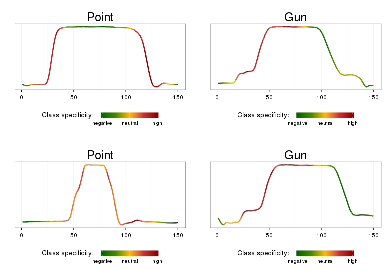
Note, that the time series ranges highlighted by the approach correspond to distinctive class features: class Gun is characterized the most by articulated movements for prop retrieval and aiming, class Point is characterized by the ‘overshoot’ phenomenon and simple (when compared to Gun) movement before aiming.
Note, that the default choice for the best parameters validation on TEST data is a parameters set corresponding to the shortest sliding window, which you may want to change - for example to choose the point whose neighborhood contains the highest density of sampled points.
Also note that code implements 5 ways the TF (term frequency value) can be computed:
double tfValue = Math.log(1.0D + Integer.valueOf(wordInBagFrequency).doubleValue());
// double tfValue = 1.0D + Math.log(Integer.valueOf(wordInBagFrequency).doubleValue());
// double tfValue = normalizedTF(bag, word.getKey());
// double tfValue = augmentedTF(bag, word.getKey());
// double tfValue = logAveTF(bag, word.getKey());
For many datasets, these yield quite different accuracy.
The normalization threshold (used in SAX discretization) is also quite important hidden parameter -- changing it from 0.001 to 0.01 may significantly change the classification accuracy on a number of datasets where the original signal standard deviation is small, such as Beef.
Finally, note, that when cosine similarity is computed within the classification procedure, it may happen that its value is the same for all classes. In that case, the current implementation considers that the time series was missclassified, but you may want to assign it to one of the classes randomly.
The following table was obtained in automated mode when using DiRect-driven parameters optimization scheme. Note, that the minimal CV error is the same for a number of parameter combinations, the sampler breaks ties by choosing a parameters set with the smallest sliding window.
| Dataset | Classes | Length | Euclidean 1NN | DTW 1NN | SAX-VSM |
|---|---|---|---|---|---|
| 50words | 50 | 270 | 0.3692 | 0.3099 | 0.3736 |
| Adiac | 37 | 176 | 0.3887 | 0.396 | 0.4169 |
| Arrowhead | 3 | 495-625 | 0.5029 | 0.5314 | 0.3429 |
| ARSim | 2 | 500 | 0.4890 | 0.4035 | 0.4405 |
| Beef | 5 | 470 | 0.4667 | 0.5000 | 0.2333 |
| CBF | 3 | 128 | 0.1478 | 0.0033 | 0.0044 |
| ChlorineConcentration | 3 | 166 | 0.3500 | 0.3516 | 0.3354 |
| CinC_ECG_torso | 4 | 1,639 | 0.1029 | 0.3493 | 0.2913 |
| Coffee | 2 | 286 | 0.2500 | 0.1786 | 0.0000 |
| Cricket | 2 | 308 | 0.0510 | 0.0102 | 0.0910 |
| Cricket_X | 12 | 300 | 0.4256 | 0.2231 | 0.3077 |
| Cricket_Y | 12 | 300 | 0.3564 | 0.2077 | 0.3180 |
| Cricket_Z | 12 | 300 | 0.3795 | 0.2077 | 0.2974 |
| DiatomSizeReduction | 4 | 345 | 0.0654 | 0.0327 | 0.1209 |
| Earthquakes | 2 | 512 | 0.3022 | 0.295 | 0.2518 |
| ECG200 | 2 | 96 | 0.1200 | 0.2300 | 0.1400 |
| ECGFiveDays | 2 | 136 | 0.2033 | 0.2323 | 0.0012 |
| ElectricDevices | 7 | 96 | 0.4559 | 0.3298 | 0.3739 |
| FaceAll | 14 | 131 | 0.2864 | 0.1923 | 0.2450 |
| FaceFour | 4 | 350 | 0.2159 | 0.1705 | 0.11364 |
| FacesUCR | 14 | 131 | 0.2307 | 0.0951 | 0.1088 |
| Fish | 7 | 463 | 0.2171 | 0.1657 | 0.0171 |
| FordA | 2 | 500 | 0.3136 | 0.2758 | 0.18561 |
| FordB | 2 | 500 | 0.4037 | 0.3407 | 0.3309 |
| GunPoint | 2 | 150 | 0.0867 | 0.0933 | 0.0133 |
| HandOutlines | 2 | 2,709 | 0.1378 | 0.1189 | 0.0703 |
| Haptics | 5 | 1,092 | 0.6299 | 0.6234 | 0.5844 |
| InlineSkate | 7 | 1,882 | 0.6582 | 0.6164 | 0.5927 |
| ItalyPowerDemand | 2 | 24 | 0.0447 | 0.0496 | 0.0894 |
| Lighting2 | 2 | 637 | 0.2459 | 0.1311 | 0.2131 |
| Lighting7 | 7 | 319 | 0.4247 | 0.2740 | 0.3973 |
| MALLAT | 8 | 1,024 | 0.0857 | 0.0661 | 0.1992 |
| Mallet | 8 | 256 | 0.0346 | 0.0236 | 0.0351 |
| MedicalImages | 10 | 99 | 0.3158 | 0.2632 | 0.5158 |
| MoteStrain | 2 | 84 | 0.1214 | 0.1653 | 0.1246 |
| NonInvasiveFetalECG_Thorax1 | 42 | 750 | 0.1710 | 0.2097 | 0.2921 |
| OliveOil | 4 | 570 | 0.1333 | 0.1333 | 0.1333 |
| OSULeaf | 6 | 427 | 0.4835 | 0.4091 | 0.0744 |
| Passgraph | 2 | 364 | 0.3740 | 0.2901 | 0.3053 |
| Shield | 3 | 1,179 | 0.1395 | 0.1395 | 0.1085 |
| SonyAIBORobotSurface | 2 | 70 | 0.3045 | 0.2745 | 0.3062 |
| SonyAIBORobotSurfaceII | 2 | 65 | 0.1406 | 0.1689 | 0.08919 |
| StarLightCurves | 3 | 1,024 | 0.1512 | 0.2080 | 0.0772 |
| SwedishLeaf | 15 | 129 | 0.2112 | 0.0503 | 0.2784 |
| Symbols | 6 | 398 | 0.1005 | 0.0067 | 0.1085 |
| SyntheticControl | 6 | 60 | 0.1200 | 0.0000 | 0.0167 |
| Trace | 4 | 275 | 0.2400 | 0.0000 | 0.0000 |
| Two_Patterns | 4 | 128 | 0.0933 | 0.0957 | 0.0040 |
| TwoLeadECG | 2 | 82 | 0.2529 | 0.0957 | 0.0141 |
| uWaveGestureLibrary_X | 8 | 315 | 0.260748 | 0.272473 | 0.3230 |
| uWaveGestureLibrary_Y | 8 | 315 | 0.338358 | 0.365997 | 0.3638 |
| uWaveGestureLibrary_Z | 8 | 315 | 0.350363 | 0.3417 | 0.3565 |
| Wafer | 2 | 152 | 0.0045 | 0.0201 | 0.0010 |
| WordsSynonyms | 25 | 270 | 0.3824 | 0.3511 | 0.4404 |
| Yoga | 2 | 426 | 0.1697 | 0.1637 | 0.1510 |